A repository to keep track of random little things I learned or thought about each day.
The Cosmic Dipole Problem (2023/11/29)
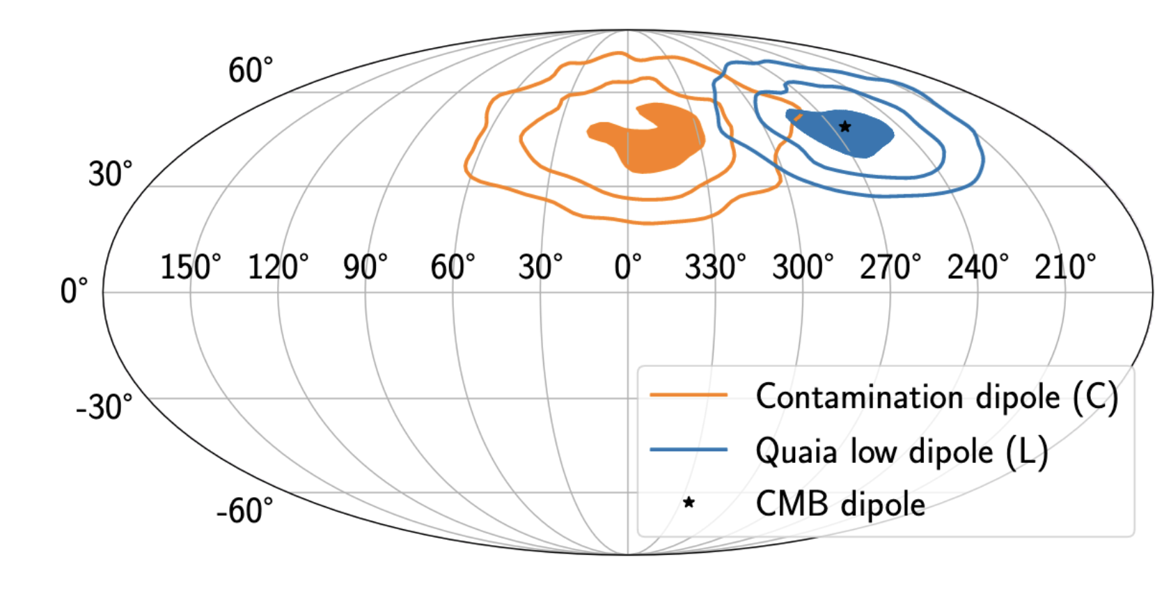
CMB features a dipole anisotropy which is interpreted as our motion relative to the cosmic rest frame. If this interpretation is correct, one expects other probe of this relative motion to feature the same cosmic dipole. However measurements from radio galaxies and quasars have presented some discrepancies in the magnitude of the cosmic dipole (see, e.g., (Peebles 2022; Kumar Aluri et al. 2023) for reviews).
A new analysis by (Mittal, Oayda, and Lewis 2023) has argued otherwise. They used 1.3 million quasars from the recently-released Quaia quasar catalogue and found that the previous discrepancies are likely due to contaminations near the Galactic Plane, and as they exclude the contaminated samples, they arrive at a result consistent both in direction and magnitude with the CMB dipole.
Observation matrix (2023/11/13)
Observation matrix, \(M\), is defined as
\begin{equation} m_{\rm out} = M m_{\rm in}. \end{equation}
The sky signal observed by detectors, \(s\), is given by
\begin{equation} s = Pm_{\rm in}, \end{equation}
where \(P\) is the pointing matrix. It can be solved by
\begin{equation} m = (P^{T}N^{-1}P)^{-1}P^TN^{-1}s \equiv Bs, \end{equation}
where \(N\) is the noise covariance matrix. One may want to apply additional filtering to deproject a set of time-domain templates, given as columns in \(F\) with
\begin{equation} Z = 1 - F(F^TN^{-1}F)F^TN^{-1}, \end{equation}
which represents deprojecting best-fit match to given set of templates. As a result,
\begin{equation} m_{\rm out} = BZs = BZPm_{\rm in}. \end{equation}
Therefore, the observation matrix is given by
\begin{equation} M = BZP = (P^{T}N^{-1}P)^{-1}P^TN^{-1}(1 - F(F^TN^{-1}F)F^TN^{-1})P. \end{equation}
Blackhole Superradiance (2023/11/13)
Superradiance is a phenomenon occurring when a wave interacts with a rotating object that has dissipative or absorptive properties. This interaction can cause the incoming wave to gain energy. For example, in a classical scenario, if a ball strikes a rotating cylinder, the ball can gain energy if the cylinder’s rotation speed exceeds the ball’s speed. Conversely, the ball loses energy if the cylinder rotates more slowly.
In astrophysics, blackhole is a perfect absorber, and a rotating blackhole, i.e., Kerr blackhole, will exhibit superradiance. If the incoming wave comes from a massless scalar field, it will have its energy boosted similar to the example of the ball. If the incoming wave comes from a massive scalar field, on the other hand, the massive field will be bound by the gravitational potential of the blackhole and form a bound state very much like a hydrogen atom. When a wave gets amplified by the blackhole through superradiance, it remains trapped in the bounded state and will keep getting amplified; this leads to a runaway growth of a cloud of particles around the blackhole, and as a result, the blackhole spin gets slowed down. As the dynamical time for the superradiance is much shorter than the lifetime of the blackhole, it will have significant impact on the evolution of the blackhole. Superradiance with massive particles therefore predicts a specific population of blackhole spins (with more low spin than high spin blackholes); this can be tested with observations from gravitational wave observatories such as LIGO.
Source: https://youtu.be/DJPFPs2kDxM?si=vgtjAIvb8EhHC6HP
Symbolic Tracing (2023/01/25)
After spending several hours reading jax’s documentation. I have finally
grasped the basic idea of it. I will try to summarize it in words. It is built
upon an elegant concept which I call function reinterpretation. The idea is
that, given an unknown implementation of a function, one can define a
transformation that reinterprets the implementation of the function without
knowing its details as long as the underlying function is composable of a
well-defined set of primitive functions that we have provided. It sounds like
magic, but it is indeed feasible and lies at the heart of jax.
jax implements this by passing in a special object known as the Tracer to
the function to obtain a specific functional Trace of our target. Intuitively,
this is like attaching a mini camera to our input variable so it can observe the
system and trace out its inner workings.
To achieve this, first we need to design our primitives such that their
evaluation can be intercepted and routed to our target Trace object which
encapsulates the specific function reinterpretation that we want to do. We then
define a corresponding Tracer object that can be used to perform (or realize)
the Trace transformation. Tracer also carries important data relevant to the
specific tracing analysis. When we pass these tracers into the function we are
probing, our tracers will trigger a series of primitive function calls which are
then routed to our Trace object, which defines how to reinterpret
each specific primitive function in terms of custom operations on the “payload”
of our Tracer. To give a specific example, suppose our function contains an
addition of two variables, such as
def target(a, b):
    c = a + b
    d = c + a
    return d
and that we want to map all additions inside our target function to
multiplications, we can define two Tracer objects that carry payload of a,
b, respectively. When our Trace intercepts the calls from “addition”
primitives, it then takes the two tracer arguments, multiplies their payload and
promotes it to another Tracer object with a payload of a*b to proceed to the
subsequent computations. At the end of the function call, we will get a tracer
object as the return. We can then simply read off its payload which represents
the result of an reinterpretation of our target function that turns addition
into multiplication. If we redefine the entire process as a new function, such as
the following pseudocode,
def add2mul(func):
    def f(a, b):
        return func(Tracer(payload=a), Tracer(payload=b)).payload
    return f

transformed_target = add2mul(target)
We have effectively transformed our target function into a different function by modifying its inner computation without actually knowing its implementation details!
- Useful resources
- Pytorch symbolic tracing paper: https://arxiv.org/pdf/2112.08429.pdf
- Explanation of jax core: https://jax.readthedocs.io/en/latest/autodidax.html
- Lightweight moduler staging: https://web.stanford.edu/class/cs442/lectures_unrestricted/cs442-lms.pdf